Teacher's Guide: Return

Overview

The introduction of return statements in this lesson is an important step towards accessing the full functionality of custom functions. Return statements themselves are conceptually simple and straightforward to use. The most challenging part of writing functions that return values is the code that generates those values. As a result, the bulk of student work for this lesson will be applying knowledge and honing skills developed in previous lessons.

More about the lesson

Custom functions can be used to perform a wide variety of tasks. The previous lesson emphasized the use of functions to perform tasks that involved animation, such as repositioning a sprite or drawing a square. With the introduction of return statements, this lesson shows how to use functions to perform many other useful tasks, such as carrrying out computations and creating objects.

The previous lesson described how to use arguments to pass information from the main part of the program to a function. Return statements simply pass back information from the function back to the main part of the program. Note that in the Pencil Code environment, return does not appear as an option in block mode, so it must be typed using text mode.

The previous lesson provided a number of motivations for defining custom functions which continue to be relevant here, such as facilitating code reuse and simplifying code maintenance. It may be useful to point out to students that functions can be seen as predefined utilities, either for frequently repeated tasks, or alternatively for tasks that may not be performed frequently, but that require many lines of code and/or complicated calculations. By defining a function, students create a utility that they can use again and again—especially after they learn to create their own Libraries, as shown in the Script Recycling! lesson.

Notes to activities

The return statement itself is the easy part of writing a custom function. The challenge is coming up with the algorithm that does the actual work or computation. Thus, the activities in this lesson all involve return statements, but they are primarily designed to give students opportunities to work on algorithms and develop computational thinking skills, building on knowledge of language features developed in previous lessons.

The MathExamples activity explicitly instructs students to test their functions using a variety of relevant test values, to ensure that the function is robust and accuratew. Such testing is critical for all functions. Emphasis should be place on thinking through what "relevant" means for each function. For an absolute value function, for example, one should test at least one positive number, one negative, and zero. For a rounding function, students should consider negative as well as positive numbers, and integer values as well as fractional values. In general, testing should include boundary cases as well as values inbetween the boundaries.

Testing functions in this manner is called unit testing, a level of software testing where the smallest testable part or components are evaluated. The purpose is to validate that each unit of the software (here, the functions) performs as designed.

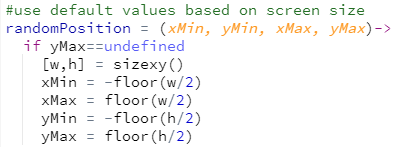
A potentially useful extention to the RandomPosition activity is to let the caller specify a region from which to select the random variables. While two points would suffice, students will likely find it easier to provide four values as arguments, xMin, xMax, yMin, yMax. One can use default values provided by sizexy, using conditional logic at the head of the function definition. For example,

The MakeLabel activity draws on jQuery techniques used to create a reference to a label, introduced in Label Recycling! For this function to be useful beyond more than a single function call, it needs to generate a unique id property for each label constructed. Encourage students to come up with their own algorithms. A simple approach is to base the ID on large random number, e.g., id: "id"+random(999999) (where the "id"+ is used to convert the number into a string that can be used as a valid property key, i.e., not starting with a number). Technically speaking, however, this approach does not guarantee unique labels, though the odds are in your favor, . A straightforward and effective alternative solution is to create timestamps for each new label's ID, e.g., id: "id"+Date.now().

The use of the jQuery (i.e., $) function necessitates animation-queue considerations. Discourage students from including calls to await done defer() inside of functions definitions. Instead, structure scripts so that calls to await done defer() either precede or follow calls to the custom function.

Additional activities

• PersonalDesmos: The MathPlots activity provided in the notes to the Custom Functions! lesson instructed you to write variants of moveto and jumpto to facilitate drawing graphs of mathematical functions in Pencil Code. In this graphing activity, tackle the same task in a different way. Write a function that transforms a coordinate that you would graph in math class to a new set of x and y values that looks good on the computer screen. Then you can use the standard Pencil Code movement functions moveto and jumpto to plot the graph of transformed values.
  

  More specifically, define a function called transform that accepts the arguments needed to carry out the computations, including an array of two values representing a coordinate that you want to transform, a scaling factor (or perhaps two, if you want to scale x and y differently), and x- and y-offsets, to specify where the origin of the underlying graph should appear with respect to Pencil Code's origin at the center of the screen.

  Begin by choosing a function to graph, such as the cubing function, a rational functions, or the sine function. Note that you can (and should) define the mathematical relationships you want to graph using custom functions., too. For example, a quadratic function could be defined as f=(x)-> return x*x + 2*x + 1. Pre-transformed coordinates can then be expressed as [x,f(x)].

• BezierCurve: Thus far in this course, students have largely been limited to drawing curved shapes using the rt and lt functions with two arguments, e.g., rt 180, 200. A more sophisticated approach makes use of a technique know as a quadratic bezier curve, which is a form of linear interpolation. Numerous online resources explore these concepts in depth; they have many applications, including . A fantastic starting point for students willing to put in a little time is provided by the Introduction to Animation lessons of Khan Academy's Pixar In A Box curriculum. Most other resources are much more technical. This detailed web resource is fairly exhaustive; students may find it most valuable for the interactive widgets it provides for exploring Bezier curves. Teachers and students with more advanced backgrounds will likely find the relevant Wikipedia page useful. It highlights the fact that quadratic Bezier curves match the curves formed by the StringArt programs students likely first coded in the Coordinates! lesson and revisited in Chase Other Sprites!.

  

  A quadratic Bezier curve is a nonlinear path traced between two points, Pstart and Pend, with the curvature determined by the selection of a third, "control" point, Pcontrol. Expressed parametrically in vector notation, the path is given by the set of points given by B(t),

  B(t) = Pcontrol + (1-t)2(Pstart - Pcontrol) + t2(Pend - Pcontrol)

  as t varies from 0 to 1. Students will likely wish to work with the x and y values of each coordinate separately. These are each computed analagously, also as a function of t:

  x(t) = xcontrol + (1-t)2(xstart - xcontrol) + t2(xend - xcontrol)

  In this activity, students should write a function that generates a set of points following a quadratic bezier path. At a minimum, the function must take three points as arguments (expressed as arrays—within the function use array destructuring to access the x and y values separately). The function should return an array of coordinates, which can then be utilized to plot the curve. Combine paths to come up with an interesting new design!

  

• VectorAlgebra: The previous exercise initially provided the following formula for computing the coordinates in the quadratic Bezier curve:

  B(t) = Pcontrol + (1-t)2(Pstart - Pcontrol) + t2(Pend - Pcontrol)

  This equation illustrates two basic operations of vector algebra, scalar multiplication and vector addition. The term "vector" has specialized meaning in math and physics, but for the current purpose we can simply equate the term "vector" with "coordinate". Scalar multiplication allows us to multiply (scale) both the x and y values of a coordinate by a real number. Vector addition facilitates adding together the x values and y values of two coordinates. Both of these vector algebra operations generate a new point. For example,

  (2,5) + (-3,4) = (-1,9)   and    3 × (2,5) = (6,15)

  The goal of this activity is to code an alternative solution to the BezierCurve activity which relies on vector math, rather than separately computing the x and y values for each point in the Bezier curve path. (In fact, the the illustrated solution for the BezierCurve activity takes this approach.) To complete this activity, you will need to define your own scalar multiplication and vector addition functions, and incorporate them into a modified version of the BezierCurve compute the array of Bezier curve coordinates. Your scalar multiplication function should take two arguments, a number and a coordinate, and it should return the scaled coordinate. Vector addition should likewise take two arguments—the coordinates, expressed as arrays—and return the summed values, also as an array. Hint: for the Bezier curve task, you will probably find it helpful also to code a vector subtraction function. If you were to name your scalar multiplication and vector addition functions vMult and vSum, respectively, then this difference function could be coded as:

  

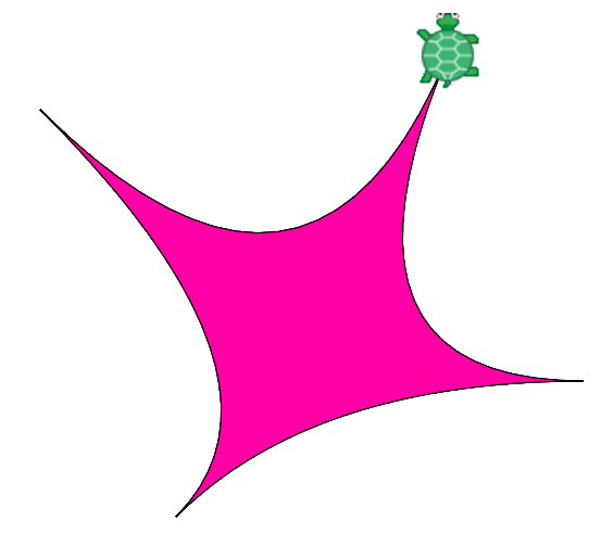
• CubicBezier: Bezier curves can be created with additional control points, allowing for greater control of the shape of a curve, such as the two curves that make up the sides of the following illustration:

  

  Recall that a quadratic Bezier curve is computed based on two end points and a control point. Cubic Bezier curves are computed based on the same underlying logic, but they have two control points.

  Some derivations of cubic Bezier curves are mathematically complex. Thankfully, the computations can be simplified by making use of the formulas (i.e., the functions) already derived to compute the quadratic Bezier curve. This is done as follows:

  • Let qB be a function that computes a set of points tracing a quadratic bezier curve. This function takes three arguments: the start point, the control point, and the end point (in that order).
  • Denote the points for a cubic Bezier curve p0, p1, p2, and p3, where p0 is the start point and p3 is the end point.
  • The points on the path of the cubic Bezier curve are given by a linear interpolation of corresponding points in the arrays of points generated from calls to qB(p1,p2,p3) and qB(p2,p3,p4). In pseudocode, this cubic bezier function can be expressed thus:
    cB(p0,p1,p2,p3) = (1-t)×qB(p0,p1,p2) + t×qB(p1,p2,p3)

    As before, t varies from 0 to 1.

  The vector algebra functions defined in the previous exercise will faciliate turning this pseudocode into Coffeescript.

• ClosestSprite: Pencil Code provides a closest function that returns the sprite closest to a given sprite or location. This function, which requires working with jQuery collections, was introduced in the Calling All $(.turtle)s!) lesson.

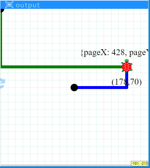
  To goal of this activity is to define your own closest function. Like the built-in version, it should take several arguments, including an array of sprites and also a target (either a location, specified as an array, or another sprite), and return the sprite (or location array) that is closest to the target. Illustrate that your function works by creating an array of randomly positioned turtles, and highlighting the ones closest to different parts of the screen, such as the center and the corners.


• CoordConverter: Recall that HTML Coordinates are an alternative to the center-based coordinates (i.e., with the origin in the center of the screen) we typically make use of in the Pencil Code environment. HTML coordinates place the origin at the top-left corner of the screen, and have positive x and y values going across and down the screen. Though we typically do our work in center-based coordinates, behind the scences, Pencil Code uses HTML Coordinates, because that's what the underlying graphcis features in HTML use.

  HTML coordinates are stored in Pencil Code as objects, such as {pageX:785, pageY:283}; you can easily generate an example yourself by calling random(position). Write a utility function convertHtmlToLocal which converts an HTML coordinates object to an array of the more familiar center-based coordinates. Also write an inverse function, convertLocalToHtml, which takes an array of center-based coordinates and converts it into an HTML-coordinates object. Try to come up with a clever way to demonstrate that your functions work correctly!



• RandomArrays: code a function randoms that generates an array of random values, which can be either numbers or strings. The function should accept three arguments: (1) the number, n, of values to choose, (2) an array of values, values, from which to choose (which you might set to a default value, such as [1..100]), and (3) a boolean value, replacement, that indicates whether numbers should be chosen with or without replacement (with default value false).

  When working on coding the replacement part of the code, it may be helpful to revisit the UniqueRandNum activity in the PushPop! lesson, which described the use of the in keyword to determine whether a value exists in an array. Additionally, note that, because colors are represented by strings, your function can be used to choose unique random colors. For example, you could define your own array of colors, or simply refer to the built-in array jquery.turtle.colors, which contains all the predefined HTML colors.

• PenPlus: Pencil Code does not provide a direct means to determine whether the turtle's pen is currently down, or to determine the color and thickness of the current pen setting. However, when writing functions, it can be useful to be able to access this information. For example, many of the functions we create to carry out animations result in changes to a turtle's pen status, compared to what it was before the function call. Typically unintended, these changes in a turtle's "status" caused by the function are known as side effects. Good coding style dictates that functions should be defined in such a way as to minimize side effects.

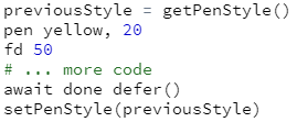
  For this activity, write functions that facilitate getting and setting the turtle's pen characteristics. Do this by accessing the turtle's css properties turtlePenDown and turtlePenStyle. Recall that we can access these properties using expressions such as turtle.css("turtlePenDown") and we can set them using statements such as turtle.css("turtlePenDown":"up"). Begin your work by exploring these properties to ascertain the possible values that they can take. Based on your findings, write functions getPenStatus (for whether it is up or down), getPenStyle, setPenStatus, and setPenStyle. For this last one, you set the pen style using the output from a prior call to getPenStyle, i.e.,

  

  Put these functions to work by embedding them in a modified drawRandomSquare function that creates a randomly sized, randomly located, randomly oriented, and randomly colored square, but afterwards returns the turtle to its original starting position, orientation, and pen status.

• CheckSpeed: Define a function that returns a turtle's current speed setting. This function should take a single argument which specifies which turtle's speed to check. The information needed to write this function is in the turtle's css property turtleSpeed. However, there is a complication. The value returned by the css can either be a numeric value representing the turtle's speed (what we want), but it can also be the string 'turtle'. This latter result is the return value when the referenced turtle is the default turtle, or when the referenced turtle is another turtle but that turtle is using the default speed. In these cases, you will need to compute and return the value 1000/jQuery.fx.speeds.turtle.

Beyond the lesson

Implicit return statements

Every function, whether or not it explicitly includes a return statement, returns a value. If a function definition does not include an explicit return statement, the return statement is defined implicitly as the value of the expression on the last line of the function is returned.

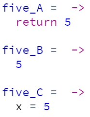
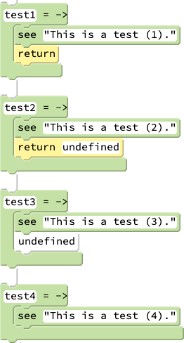
To illustrate, consider the following example function definitions, each of which, when called, returns the value 5:

The fact that the third example returns 5 owes to the fact that the CoffeeScript compiler tries to make sure that all statements in the language can be used as expressions (meaning, each statement, even those involving assignment, have a value). Thus, in general, an expression such as x = 5 not only completes the variable assignment of 5 to x, but the expression itself has a value, which in this case is the value of x after the assignment (i.e., 5). (As a result, even a statement such as y = (x=5)*5 is valid in CoffeeScript: it assigns 5 to x and then 25 to y, all in a single statement!)

An implication of implicit return statements is that all functions return a value. But what if a function is not intended to return a value, but simply to carry out a task, as with all the activities and examples of the Custom Functions! lesson? The solution is to return the value undefined—the special value (and data type, with the same name) to which variables that have not been initialized are set.

The following examples illustrate several ways that a function may be coded to return undefined:

The final example above returns undefined because see itself returns undefined.

Function chaining

Function chaining is a JavaScript language feature that allows multiple functions calls on the same object consecutively. In practical terms, function chaining facilitates combining multiple lines of code into one. For example, consider the following simple script:

The following script combines these five lines into one. The only required change to the statements in the previous example is addition of explicit parentheses, needed to ensure that the compiler correctly interprets the arguments.

Function chaining is possible because of return statements. The initial call to the constructor (itself a special type of function that is invoked using the reserved word new) returns a reference to the newly created Turtle object. We assign this to r in both examples above. But in the latter example, we take advantage of the fact that the reference created by the constructor call can be directly accessed using dot notation. (The fact that the reference was assigned to r is irrelevant to this action.) The call to the Turtle object's pen method not only sets the pen, but iself returns a reference to the Turtle object itself, enabling us to use dot notation to continue the function chain.

Function chaining can be used whenever the output of a function is an object that has its own methods (i.e., functions associated with the instance of that object). It is strongly supported by the jQuery library, which underlies most animation in the Pencil Code environment. As a result, most built-in Pencil Code functions support chaining. (speed is perhaps the most notable exception.)

CoffeeScript layers in an additional features that can make chaining even easier to use. As illustrated in the following example, sucessive use of the dot operator can be placed on the following line of code:

Students can make use of function chaining at this point, using built-in object types. However, coding custom objects that support chaining requires a deeper understanding of methods and specificially use of the reserved word this. These features will be explored further in the Methods! lesson.